导入需要的库
1 | from __future__ import absolute_import |
下载并读取语料库中的数据
首先运行如下代码,下载语料库。1
2
3
4
5
6
7
8
9
10
11
12
13
14
15
16
17
18
19
20
21
22
23
24# 第一步: 在下面这个地址下载语料库
url = 'http://mattmahoney.net/dc/'
def maybe_download(filename, expected_bytes):
"""
这个函数的功能是:
如果filename不存在,就在上面的地址下载它。
如果filename存在,就跳过下载。
最终会检查文字的字节数是否和expected_bytes相同。
"""
if not os.path.exists(filename):
print('start downloading...')
filename, _ = urllib.request.urlretrieve(url + filename, filename)
statinfo = os.stat(filename)
if statinfo.st_size == expected_bytes:
print('Found and verified', filename)
else:
print(statinfo.st_size)
raise Exception(
'Failed to verify ' + filename + '. Can you get to it with a browser?')
return filename
# 下载语料库text8.zip并验证下载
filename = maybe_download('text8.zip', 31344016)
运行如下代码,将语料库转化为列表,并打印语料库单词长度以及前100个单词。1
2
3
4
5
6
7
8
9
10
11
12
13
14# 将语料库解压,并转换成一个word的list
def read_data(filename):
"""
这个函数的功能是:
将下载好的zip文件解压并读取为word的list
"""
with zipfile.ZipFile(filename) as f:
data = tf.compat.as_str(f.read(f.namelist()[0])).split()
return data
vocabulary = read_data(filename)
print('Data size', len(vocabulary)) # 总长度为1700万左右
# 输出前100个词。
print(vocabulary[0:100])
打印输出结果如下图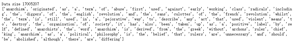
语料库预处理,制作词表
1 | # 第二步: 制作一个词表,将不常见的词变成一个UNK标识符 |
说明:
data : 转化为索引的数据集
count : 词频统计
dictionary : 单词到索引的映射
reverse_dictionary : 索引到单词的映射
上述代码打印结果如下图:
CBOW
定义模型生成 batch 的函数
1 | # 第三步:定义一个函数,用于生成cbow模型用的batch |
训练
1 | num_steps = 100001 |
可视化
1 | # Step 6: 可视化 |
运行代码后,生成结果如下图: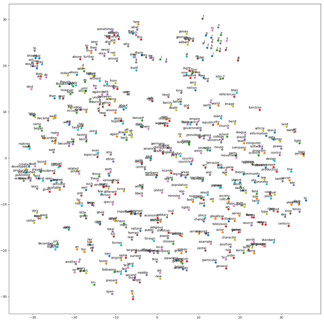
完整代码
1 | # coding: utf-8 |
Skip-gram
制作训练集
1 | # 我们下面就使用data来制作训练集 |
我们运行如下代码,试着打印一下生成的训练集的 batch1
2
3
4
5
6
7
8# 默认情况下skip_window=1, num_skips=2
# 此时就是从连续的3(3 = skip_window*2 + 1)个词中生成2(num_skips)个样本。
# 如连续的三个词['used', 'against', 'early']
# 生成两个样本:against -> used, against -> early
batch, labels = generate_batch(batch_size=8, num_skips=2, skip_window=1)
for i in range(8):
print(batch[i], reverse_dictionary[batch[i]],
'->', labels[i, 0], reverse_dictionary[labels[i, 0]])
运行结果如下图: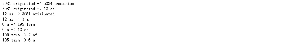
建立模型
1 | # 第四步: 建立模型. |
训练
1 | # 第五步:开始训练 |
我们可以看到最近一次的训练结果,词语的相似度越大,语义约接近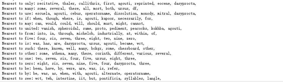
可视化
1 | # Step 6: 可视化 |
可视化结果如下图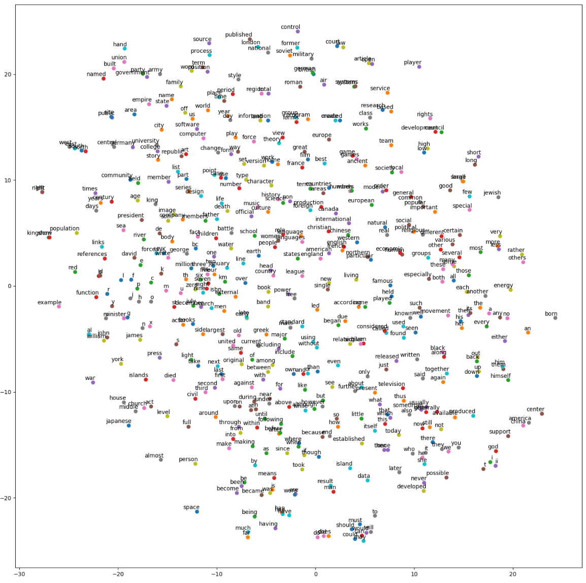
完整代码
1 | # coding: utf-8 |