数据集
载入数据集
1 | import numpy as np |
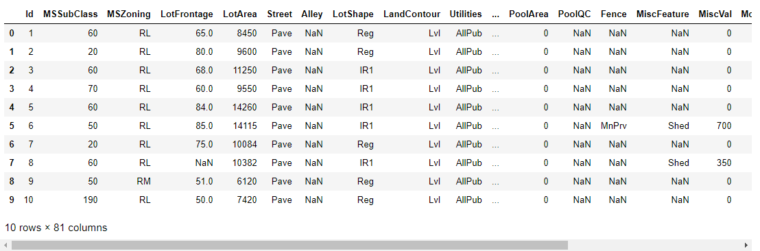
查看训练集1
train.head(10)
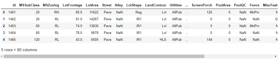
查看测试集1
train.head(10)
处理 Id 列
因为 Id 列与预测无关,现将其保存,然后从训练集和测试集中删除。1
2
3
4train_ID = train['Id']
test_ID = test['Id']
train.drop("Id", axis = 1, inplace = True)
test.drop("Id", axis = 1, inplace = True)
数据分析
- 理解问题:查看每个变量并且根据他们的意义和对问题的重要性进行哲学分析。
- 单因素研究:只关注因变量( SalePrice),并且进行更深入的了解。
- 多因素研究:分析因变量和自变量之间的关系。
- 基础清洗:清洗数据集并且对缺失数据,异常值和分类数据进行一些处理。
- 检验假设:检查数据是否和多元分析方法的假设达到一致
准备工作——我们可以期望什么?
为了了解我们的数据,我们可以分析每个变量并且尝试理解他们的意义和与该问题的相关程度。
首先建立一个 Excel 电子表格,有如下目录:
- 变量 – 变量名。
- 类型 – 该变量的类型。这一栏只有两个可能值,“数据” 或 “类别”。 “数据” 是指该变量的值是数字,“类别” 指该变量的值是类别标签。
- 划分 – 指示变量划分. 我们定义了三种划分:建筑,空间,位置。
- 期望 – 我们希望该变量对房价的影响程度。我们使用类别标签 “高”,“中” 和 “低” 作为可能值。
- 结论 – 我们得出的该变量的重要性的结论。在大概浏览数据之后,我们认为这一栏和 “期望” 的值基本一致。
- 评论 – 我们看到的所有一般性评论。
我们首先阅读了每一个变量的描述文件,同时思考这三个问题:
- 我们买房子的时候会考虑这个因素吗?
- 如果考虑的话,这个因素的重要程度如何?
- 这个因素带来的信息在其他因素中出现过吗?
我们根据以上内容填好了电子表格,并且仔细观察了 “高期望” 的变量。然后绘制了这些变量和房价之间的散点图,填在了 “结论” 那一栏,也正巧就是对我们的期望值的校正。
我们总结出了四个对该问题起到至关重要的作用的变量:
- OverallQual
- YearBuilt.
- TotalBsmtSF.
- GrLivArea.
最重要的事情——分析 “房价”
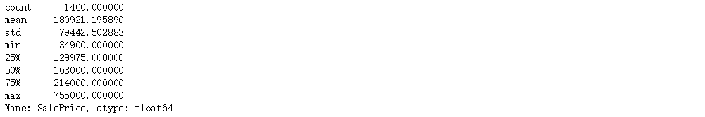
描述性数据总结
1 | train['SalePrice'].describe() |
绘制直方图
1 | sns.distplot(train['SalePrice']) |
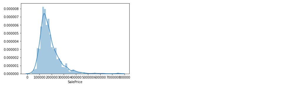
从直方图中可以看出
- 偏离正态分布
- 数据正偏
- 有峰值
数据偏度和峰度度量
1 | print("Skewness: %f" % train['SalePrice'].skew()) |

“房价” 的相关变量分析
与数字型变量的关系
Grlivarea 与 SalePrice 散点图
1 | data = pd.concat([train['SalePrice'], train['GrLivArea']], axis=1) |
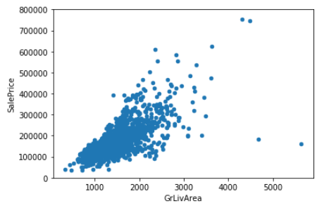
可以看出 SalePrice 和 GrLivArea 关系很密切,并且基本呈线性关系。
TotalBsmtSF 与 SalePrice 散点图
1 | data = pd.concat([train['SalePrice'], train['TotalBsmtSF']], axis=1) |
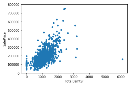
TotalBsmtSF 和 SalePrice 关系也很密切,从图中可以看出基本呈指数分布,但从最左侧的点可以看出特定情况下 TotalBsmtSF 对 SalePrice 没有产生影响。
与类别型变量的关系
OverallQual 与 SalePrice 箱型图
1 | data = pd.concat([train['SalePrice'], train['OverallQual']], axis=1) |
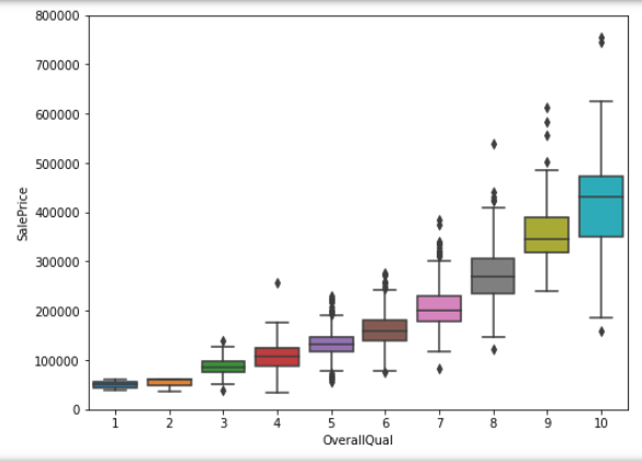
可以看出 SalePrice 与 OverallQual 分布趋势相同。
YearBuilt 与 SalePrice 箱型图
1 | data = pd.concat([train['SalePrice'], train['YearBuilt']], axis=1) |
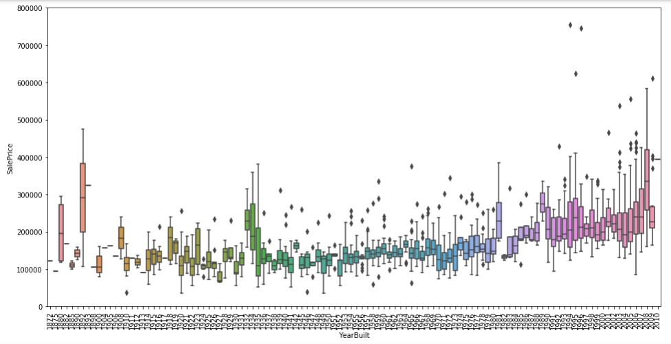
两个变量之间的关系没有很强的趋势性,但是可以看出建筑时间较短的房屋价格更高。
数据预处理
导入相关库
1 | # 导入作图用库 |
异常值
1 | fig, ax = plt.subplots() |
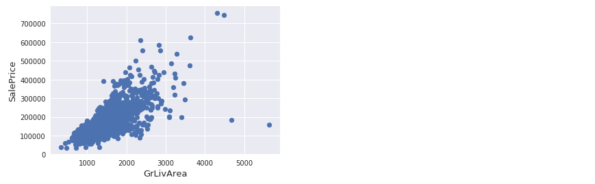
从图中可以看出:
- 有两个离群的 GrLivArea 值很高的数据,我们可以推测出现这种情况的原因。或许他们代表了农业地区,也就解释了低价。 这两个点很明显不能代表典型样例,所以我们将它们定义为异常值并删除。
- 图中顶部的两个点是七点几的观测值,他们虽然看起来像特殊情况,但是他们依然符合整体趋势,所以我们将其保留下来。
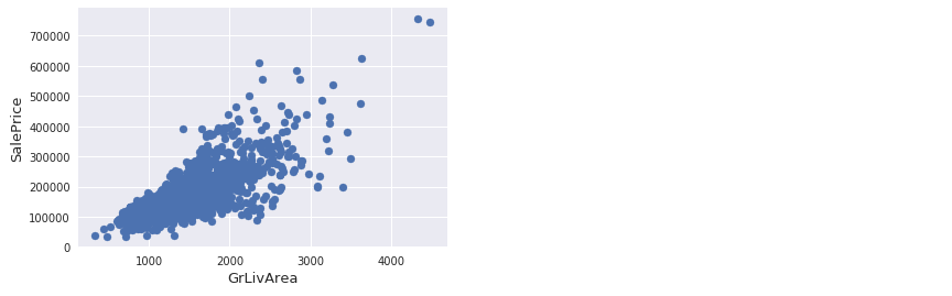
删除异常值1
2
3
4
5
6
7
8train = train.drop(train[(train['GrLivArea']>4000) & (train['SalePrice']<300000)].index)
# Check the graphic again
fig, ax = plt.subplots()
ax.scatter(train['GrLivArea'], train['SalePrice'])
plt.ylabel('SalePrice', fontsize=13)
plt.xlabel('GrLivArea', fontsize=13)
plt.show()
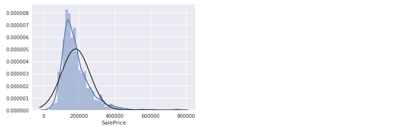
SalePrice 处理
可视化分析
绘制直方图1
2
3sns.distplot(train['SalePrice'], fit=norm)
(mu, sigma) = norm.fit(train['SalePrice'])
print( '\n mu = {:.2f} and sigma = {:.2f}\n'.format(mu, sigma))
绘制正态概率图1
2fig = plt.figure()
res = stats.probplot(train['SalePrice'], plot=plt)
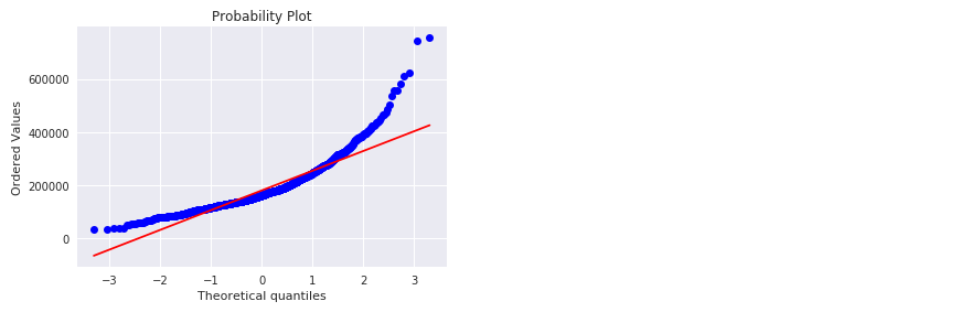
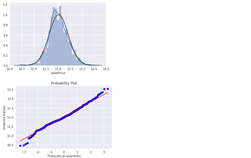
可以看出,房价分布不是正态的,显示了峰值,正偏度,但是并不跟随对角线。可以用对数变换来解决这个问题
对数变换
1 | train["SalePrice"] = np.log1p(train["SalePrice"]) |
看下处理后的图像:1
2
3sns.distplot(train['SalePrice'], fit=norm);
fig = plt.figure()
res = stats.probplot(train['SalePrice'], plot=plt)
数据合并
因为在处理相关数据时,训练集和测试集要进行相同的操作。所以我们先将 train 和 test 进行合并,处理完毕之后再分开。 train 比 test 多一列标签,我们先将其存入 y_train ,然后再合并数据。1
2
3
4
5
6ntrain = train.shape[0]
ntest = test.shape[0]
y_train = train.SalePrice.values
train.drop(['SalePrice'], axis=1, inplace=True)
all_data = pd.concat((train, test)).reset_index(drop=True)
print("all_data size is : {}".format(all_data.shape))

处理缺失值
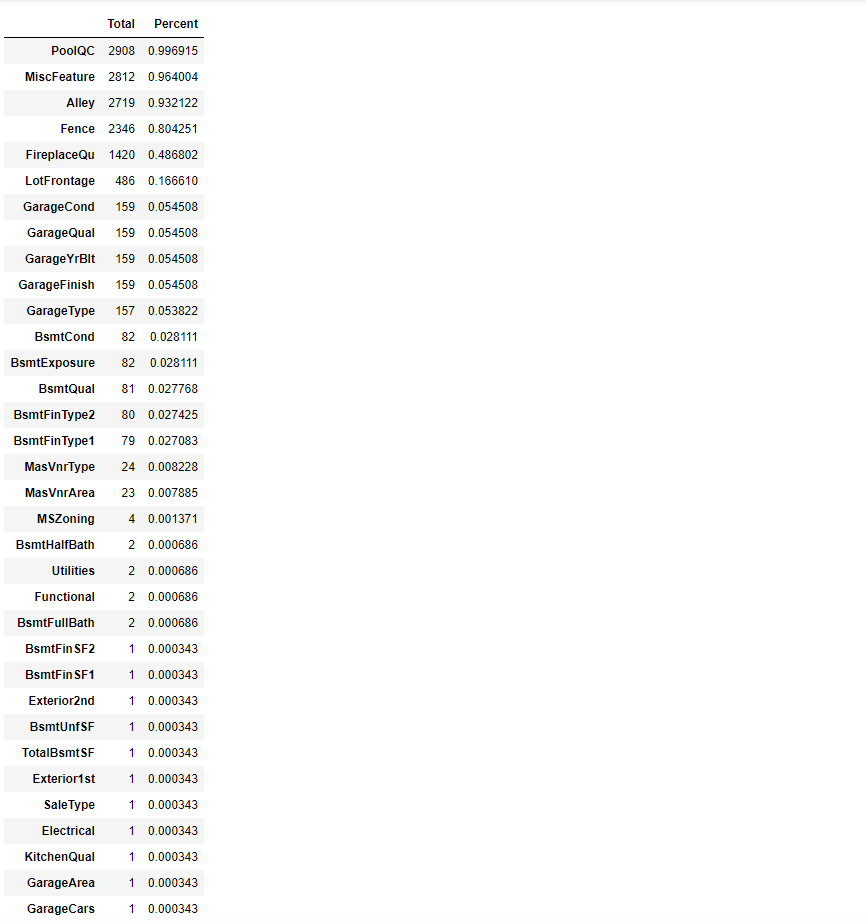
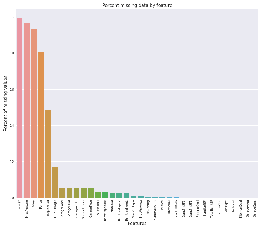
查看缺失数据
1 | total = all_data.isnull().sum().sort_values(ascending=False) |
数据处理分析
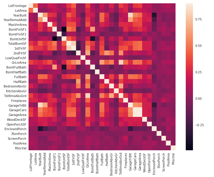
热力图
在绘制热力图之前,我们先将数据处理一下,热力图默认取整数或者浮点数据类型进行绘制,但是有些类别型数据也是用整数表示,我们将其转化一下。1
2
3
4
5
6
7all_data['MSSubClass'] = all_data['MSSubClass'].apply(str)
#Changing OverallX into a categorical variable
all_data['OverallQual'] = all_data['OverallQual'].astype(str)
all_data['OverallCond'] = all_data['OverallCond'].astype(str)
#Year and month sold are transformed into categorical features.
all_data['YrSold'] = all_data['YrSold'].astype(str)
all_data['MoSold'] = all_data['MoSold'].astype(str)
绘制图形1
2
3corrmat = all_data.corr()
plt.subplots(figsize=(12,9))
sns.heatmap(corrmat, vmax=0.9, square=True)
数据填充
- PoolQC : data description says NA means “No Pool”. That make sense, given the huge ratio of missing value (+99%) and majority of houses have no Pool at all in general.
- MiscFeature : data description says NA means “no misc feature”
- Alley : data description says NA means “no alley access”
- Fence : data description says NA means “no fence”
FireplaceQu : data description says NA means “no fireplace”
1
2for col in ("PoolQC", "MiscFeature", "Alley", "Fence", "FireplaceQu"):
all_data[col].fillna("None", inplace=True)LotFrontage : Since the area of each street connected to the house property most likely have a similar area to other houses in its neighborhood , we can fill in missing values by the median LotFrontage of the neighborhood.
1
all_data["LotFrontage"] = all_data.groupby("Neighborhood")["LotFrontage"].transform(lambda x: x.fillna(x.median()))
GarageType, GarageFinish, GarageQual and GarageCond : Replacing missing data with None
1
2for col in ('GarageType', 'GarageFinish', 'GarageQual', 'GarageCond'):
all_data[col].fillna('None', inplace=True)GarageYrBlt, GarageArea and GarageCars : Replacing missing data with 0 (Since No garage = no cars in such garage.)
1
2for col in ('GarageYrBlt', 'GarageArea', 'GarageCars'):
all_data[col].fillna(0, inplace=True)BsmtFinSF1, BsmtFinSF2, BsmtUnfSF, TotalBsmtSF, BsmtFullBath and BsmtHalfBath : missing values are likely zero for having no basement
1
2for col in ('BsmtFinSF1', 'BsmtFinSF2', 'BsmtUnfSF','TotalBsmtSF', 'BsmtFullBath', 'BsmtHalfBath'):
all_data[col].fillna(0, inplace=True)BsmtQual, BsmtCond, BsmtExposure, BsmtFinType1 and BsmtFinType2 : For all these categorical basement-related features, NaN means that there is no basement.
1
2for col in ('BsmtQual', 'BsmtCond', 'BsmtExposure', 'BsmtFinType1', 'BsmtFinType2'):
all_data[col].fillna('None', inplace=True)MasVnrArea and MasVnrType : NA most likely means no masonry veneer for these houses. We can fill 0 for the area and None for the type.
1
2all_data["MasVnrType"].fillna("None", inplace=True)
all_data["MasVnrArea"].fillna(0, inplace=True)MSZoning (The general zoning classification) : ‘RL’ is by far the most common value. So we can fill in missing values with ‘RL’
1
all_data['MSZoning'].fillna(all_data['MSZoning'].mode()[0], inplace=True)
Utilities : For this categorical feature all records are “AllPub”, except for one “NoSeWa” and 2 NA . Since the house with ‘NoSewa’ is in the training set, this feature won’t help in predictive modelling. We can then safely remove it.
1
all_data.drop(['Utilities'], axis=1, inplace=True)
Functional : data description says NA means typical1
all_data["Functional"].fillna("Typ", inplace=True)
- Electrical : It has one NA value. Since this feature has mostly ‘SBrkr’, we can set that for the missing value.
- KitchenQual: Only one NA value, and same as Electrical, we set ‘TA’ (which is the most frequent) for the missing value in KitchenQual.
- Exterior1st and Exterior2nd : Again Both Exterior 1 & 2 have only one missing value. We will just substitute in the most common string
- SaleType : Fill in again with most frequent which is “WD”
1
2for col in ('Electrical', 'KitchenQual', 'Exterior1st', 'Exterior2nd', 'SaleType'):
all_data[col].fillna(all_data[col].mode()[0], inplace=True)
数据转化
GrLivArea
绘制直方图和正态概率曲线图:1
2
3sns.distplot(all_data['GrLivArea'], fit=norm);
fig = plt.figure()
res = stats.probplot(all_data['GrLivArea'], plot=plt)

进行对数变换:1
all_data['GrLivArea']= np.log(all_data['GrLivArea'])
转换后作图如下(代码同上):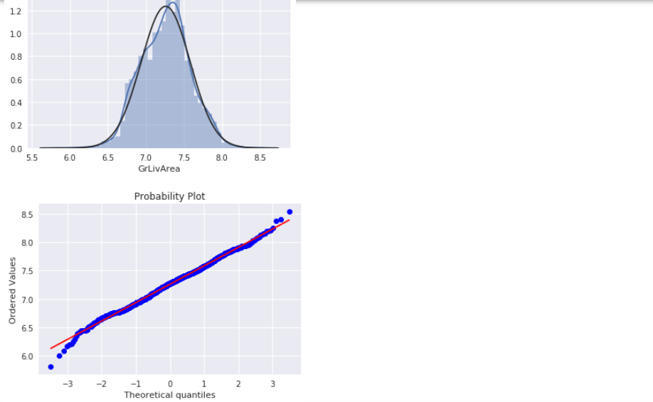
TotalBsmtSF
绘制直方图和正态概率曲线图:1
2
3sns.distplot(all_data['TotalBsmtSF'],fit=norm);
fig = plt.figure()
res = stats.probplot(all_data['TotalBsmtSF'],plot=plt)
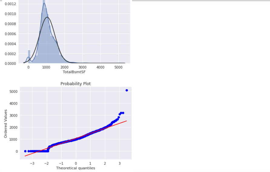
从图中可以看出:
- 显示出了偏度
- 大量为 0 的观察值(没有地下室的房屋)
- 含 0 的数据无法进行对数变换
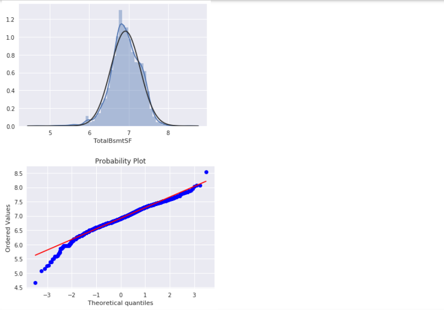
进行对数变换:1
all_data['TotalBsmtSF']= np.log1p(all_data['TotalBsmtSF'])
我们选择忽略零值,只对非零值进行可视化。1
2
3
4#histogram and normal probability plot
sns.distplot(all_data[all_data['TotalBsmtSF']>0]['TotalBsmtSF'], fit=norm);
fig = plt.figure()
res = stats.probplot(all_data[all_data['TotalBsmtSF']>0]['TotalBsmtSF'], plot=plt)
类别编码 与 虚拟变量
有些类别变量包含一些顺序的信息,比如房屋设备的评级(由低到高或者由高到低),这种我们不必采用 one-hot 编码1
2
3
4
5
6
7
8
9
10from sklearn.preprocessing import LabelEncoder
cols = ['MSSubClass', 'Street', 'Alley', 'LotShape', 'LandSlope', 'OverallQual', 'OverallCond',
'ExterQual', 'ExterCond', 'BsmtQual', 'BsmtCond', 'BsmtExposure', 'BsmtFinType1', 'BsmtFinType2',
'HeatingQC', 'CentralAir', 'KitchenQual', 'Functional', 'FireplaceQu','GarageFinish','GarageQual',
'GarageCond', 'PavedDrive', 'PoolQC', 'Fence', 'MoSold', 'YrSold']
# process columns, apply LabelEncoder to categorical features
for c in cols:
lbl = LabelEncoder()
lbl.fit(list(all_data[c].values))
all_data[c] = lbl.transform(list(all_data[c].values))
最后将类别变量转化为虚拟变量1
2all_data = pd.get_dummies(all_data)
print(all_data.shape)
拆分数据集
1 | train = all_data[:ntrain] |
模型训练
导入库
1 | from sklearn.linear_model import ElasticNet, Lasso, BayesianRidge, LassoLarsIC |
定义交叉验证策略
我们使用 cross_val_score 函数进行交叉验证。但是该函数没有打乱数据集的功能,所以我们增加了一行代码,为了在交叉验证前打乱数据集。1
2
3
4
5n_folds = 5
def rmsle_cv(model):
kf = KFold(n_folds, shuffle=True, random_state=42).get_n_splits(train.values)
rmse= np.sqrt(-cross_val_score(model, train.values, y_train, scoring="neg_mean_squared_error", cv = kf))
return(rmse)
基础模型
LASSO Regression :
该模型对于异常值比较敏感,因此我们需要使其更健壮,在进行数据建模之前我们使用 Robustscaler() 方法。1
lasso = make_pipeline(RobustScaler(), Lasso(alpha =0.0005, random_state=1))
Elastic Net Regression :
1
ENet = make_pipeline(RobustScaler(), ElasticNet(alpha=0.0005, l1_ratio=.9, random_state=3))
Kernel Ridge Regression:
1
KRR = KernelRidge(alpha=0.6, kernel='polynomial', degree=2, coef0=2.5)
Gradient Boosting Regression:
1
2
3
4GBoost = GradientBoostingRegressor(n_estimators=3000, learning_rate=0.05,
max_depth=4, max_features='sqrt',
min_samples_leaf=15, min_samples_split=10,
loss='huber', random_state =5)XGBoost:
1
2
3
4
5
6model_xgb = xgb.XGBRegressor(colsample_bytree=0.4603, gamma=0.0468,
learning_rate=0.05, max_depth=3,
min_child_weight=1.7817, n_estimators=2200,
reg_alpha=0.4640, reg_lambda=0.8571,
subsample=0.5213, silent=1,
random_state =7, nthread = -1)LightGBM:
1
2
3
4
5
6model_lgb = lgb.LGBMRegressor(objective='regression',num_leaves=5,
learning_rate=0.05, n_estimators=720,
max_bin = 55, bagging_fraction = 0.8,
bagging_freq = 5, feature_fraction = 0.2319,
feature_fraction_seed=9, bagging_seed=9,
min_data_in_leaf =6, min_sum_hessian_in_leaf = 11)