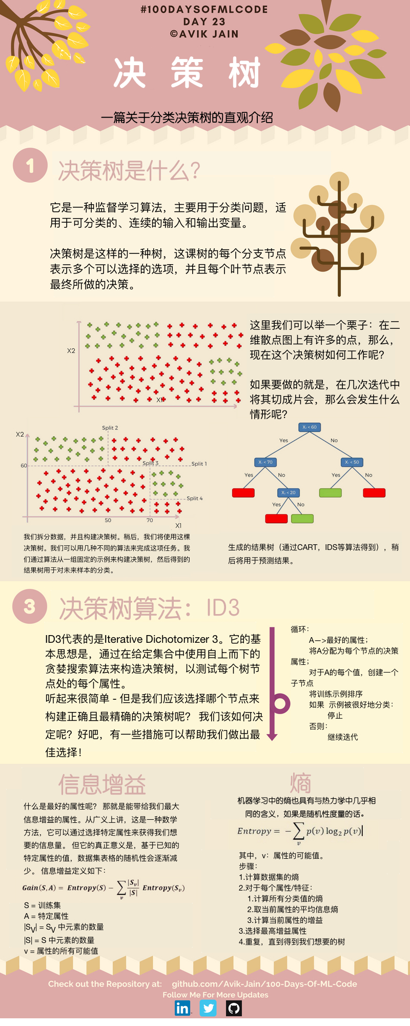
基本步骤
数据集
导入需要用到的python库
1 | import numpy as np |
导入数据集
1 | dataset = pd.read_csv('Social_Network_Ads.csv') |
将数据集拆分为训练集和测试集
1 | from sklearn.model_selection import train_test_split |
对测试集进行决策树分类拟合
1 | from sklearn.tree import DecisionTreeClassifier |
为了防止过拟合,对于决策树有时会进行剪枝处理,在分类器中我们可以通过设置参数 max_depth 和 min_samples_split 调节决策的深度与内部节点再划分所需最小样本数。
预测测试集的结果
1 | y_pred = classifier.predict(X_test) |
制作混淆矩阵
1 | from sklearn.metrics import confusion_matrix |
打印混淆矩阵,cm 结果为:1
2[[62 6]
[ 3 29]]
结果进行可视化
可视化相关代码详见另一篇文章《机器学习实战-逻辑回归》
训练集结果可视化如下图: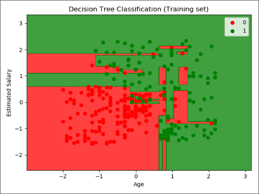
测试集结果可视化如下图: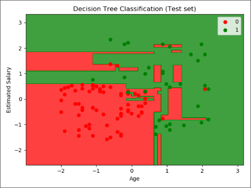
导出决策树
我们可以通过命令 pip install graphviz ,或者登陆 graphviz官网,下载相应的包。1
2
3
4
5
6
7
8
9
10
11import graphviz
from sklearn.tree import export_graphviz
dot_data = export_graphviz(classifier,
out_file=None,
feature_names=["Age", "EstimatedSalary"],
class_names=["no", "yes"],
filled=True,
rounded=True,
special_characters=True)
graph = graphviz.Source(dot_data)
graph.render('computer')
运行以上代码后,会在相对路径下生成一个 pdf 文件,图形保存在其中,如下所示: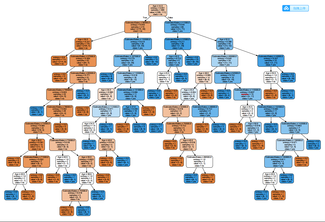
补充方法
有时候我们遇到的数据集都是离散型的非数值,这时候需要对所有的特征值做预处理,将其转化为数字,我们可以使用 sklearn.feature_extraction 中的 DictVectorizer 类,该类的输入是一个字典,相当于将字典向量化。如何操作?我们看下面的例子。
数据集
| RID | age | income | student | credit_rating | class_buys_computer |
|---|---|---|---|---|---|
| 1 | youth | high | no | fair | no |
| 2 | youth | high | no | excellent | no |
| 3 | middle_aged | high | no | fair | yes |
| 4 | senior | medium | no | fair | yes |
| 5 | senior | low | yes | fair | yes |
| 6 | senior | low | yes | excellent | no |
| 7 | middle_aged | low | yes | excellent | yes |
| 8 | youth | medium | no | fair | no |
| 9 | youth | low | yes | fair | yes |
| 10 | senior | medium | yes | fair | yes |
| 11 | youth | medium | yes | excellent | yes |
| 12 | middle_aged | medium | no | excellent | yes |
| 13 | middle_aged | high | yes | fair | yes |
| 14 | senior | medium | no | excellent | no |
数据预处理
因为要将数据转化为字典形式的列表,所以我们用 csv.reader 一行一行读取数据,并进行数据转化。1
2
3
4
5
6import csv
# 读入数据
dataset = open(r'AllElectronics.csv', 'r')
reader = csv.reader(dataset)
# 获取第一行数据(表头信息)
headers = reader.__next__()
运行命令 print(headers) 打印表头信息,得到以下结果:1
['RID', 'age', 'income', 'student', 'credit_rating', 'class_buys_computer']
1 | # 定义两个列表 |
分别打印 featureList 和 labelList 得到以下结果:1
2
3
4
5
6
7
8
9
10
11
12
13
14
15
16
17featureList:
[{'age': 'youth', 'income': 'high', 'student': 'no', 'credit_rating': 'fair'},
{'age': 'youth', 'income': 'high', 'student': 'no', 'credit_rating': 'excellent'},
{'age': 'middle_aged', 'income': 'high', 'student': 'no', 'credit_rating': 'fair'},
{'age': 'senior', 'income': 'medium', 'student': 'no', 'credit_rating': 'fair'},
{'age': 'senior', 'income': 'low', 'student': 'yes', 'credit_rating': 'fair'},
{'age': 'senior', 'income': 'low', 'student': 'yes', 'credit_rating': 'excellent'},
{'age': 'middle_aged', 'income': 'low', 'student': 'yes', 'credit_rating': 'excellent'},
{'age': 'youth', 'income': 'medium', 'student': 'no', 'credit_rating': 'fair'},
{'age': 'youth', 'income': 'low', 'student': 'yes', 'credit_rating': 'fair'},
{'age': 'senior', 'income': 'medium', 'student': 'yes', 'credit_rating': 'fair'},
{'age': 'youth', 'income': 'medium', 'student': 'yes', 'credit_rating': 'excellent'},
{'age': 'middle_aged', 'income': 'medium', 'student': 'no', 'credit_rating': 'excellent'},
{'age': 'middle_aged', 'income': 'high', 'student': 'yes', 'credit_rating': 'fair'},
{'age': 'senior', 'income': 'medium', 'student': 'no', 'credit_rating': 'excellent'}]
labelList:
['no', 'no', 'yes', 'yes', 'yes', 'no', 'yes', 'no', 'yes', 'yes', 'yes', 'yes', 'yes', 'no']
特征转化
这一步利用 DictVectorizer 类将非数值形特征转化为 0 和 1 的表示。1
2
3
4from sklearn.feature_extraction import DictVectorizer
# 把数据转换成01表示
vec = DictVectorizer()
x_data = vec.fit_transform(featureList).toarray()
通过 print(vec.get_feature_names()) 打印属性名称,并打印转化后的数据结果 x_data :1
2
3
4
5
6
7
8
9
10
11
12
13
14
15
16
17vec.get_feature_names:
['age=middle_aged', 'age=senior', 'age=youth', 'credit_rating=excellent', 'credit_rating=fair', 'income=high', 'income=low', 'income=medium', 'student=no', 'student=yes']
x_data:
[[0. 0. 1. 0. 1. 1. 0. 0. 1. 0.]
[0. 0. 1. 1. 0. 1. 0. 0. 1. 0.]
[1. 0. 0. 0. 1. 1. 0. 0. 1. 0.]
[0. 1. 0. 0. 1. 0. 0. 1. 1. 0.]
[0. 1. 0. 0. 1. 0. 1. 0. 0. 1.]
[0. 1. 0. 1. 0. 0. 1. 0. 0. 1.]
[1. 0. 0. 1. 0. 0. 1. 0. 0. 1.]
[0. 0. 1. 0. 1. 0. 0. 1. 1. 0.]
[0. 0. 1. 0. 1. 0. 1. 0. 0. 1.]
[0. 1. 0. 0. 1. 0. 0. 1. 0. 1.]
[0. 0. 1. 1. 0. 0. 0. 1. 0. 1.]
[1. 0. 0. 1. 0. 0. 0. 1. 1. 0.]
[1. 0. 0. 0. 1. 1. 0. 0. 0. 1.]
[0. 1. 0. 1. 0. 0. 0. 1. 1. 0.]]
1 | from sklearn.preprocessing import LabelBinarizer |
打印转化后的数据结果 y_data :1
2
3
4
5
6
7
8
9
10
11
12
13
14
15y_data:
[[0]
[0]
[1]
[1]
[1]
[0]
[1]
[0]
[1]
[1]
[1]
[1]
[1]
[0]]
得到的 x_data 和 y_data 直接放入模型训练即可。
回归
在回归问题中CART 算法的工作方式与之前处理分类模型基本一样,不同之处在于,现在不再以最小化不纯度的方式分割训练集,而是试图以最小化 MSE 的方式分割训练集。
决策树也能够执行回归任务,让我们使用 Scikit-Learn 的 DecisionTreeRegressor 类构建一个回归树,让我们用 max_depth = 2 在具有噪声的二次项数据集上进行训练。
生成数据集
1 | # Quadratic training set + noise |
训练模型
1 | from sklearn.tree import DecisionTreeRegressor |
生成图形
1 | from sklearn.tree import export_graphviz |
运行上述代码后,在当前文件夹下生成 regression_tree.dot 文件,需要使用命令 dot -Tpng regression_tree.dot -o regression_tree.png 将其转化为图片,如下所示: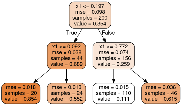
这棵树看起来非常类似于你之前建立的分类树,它的主要区别在于,它不是预测每个节点中的样本所属的分类,而是预测一个具体的数值。
预测结果可视化
1 | import matplotlib.pyplot as plt |
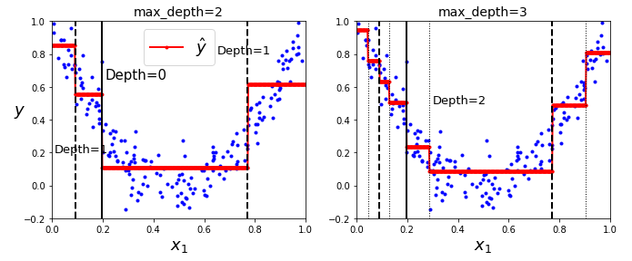
上图的左侧显示的是模型的预测结果,如果你将 max_depth=3 设置为 3,模型就会如右侧显示的那样。注意每个区域的预测值总是该区域中实例的平均目标值。算法以一种使大多数训练实例尽可能接近该预测值的方式分割每个区域。
过拟合与正则化
1 | tree_reg1 = DecisionTreeRegressor(random_state=42) |
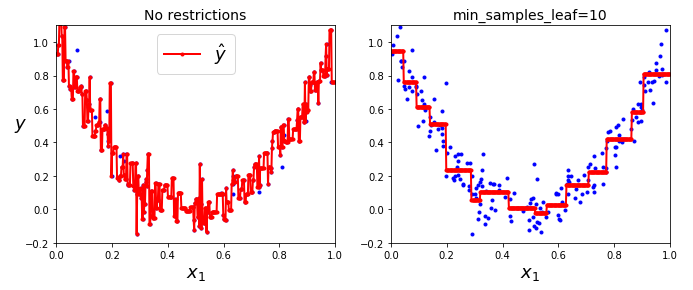
和处理分类任务时一样,决策树在处理回归问题的时候也容易过拟合。如果不添加任何正则化(默认的超参数),你就会得到上图左侧的预测结果,显然,过度拟合的程度非常严重。而当我们设置了 min_samples_leaf = 10 ,相对就会产生一个更加合适的模型了,就如右图所示的那样。
调参 ★
max_depth:最大深度min_samples_split:节点在被分裂之前必须具有的最小样本数min_samples_leaf:叶节点必须具有的最小样本数min_weight_fraction_leaf:和min_samples_leaf相同,但表示为加权总数的一小部分实例max_leaf_nodes:叶节点的最大数量max_features:在每个节点被评估是否分裂的时候,具有的最大特征数量- 增加
min_* hyperparameters或者减少max_* hyperparameters会使模型正则化。