卷积神经网络 CNN 模型

LeNET-5模型

简介

LeNet-5 出自论文 Gradient-Based Learning Applied to Document Recognition,是一种用于手写体字符识别的非常高效的卷积神经网络。

01_LeNet-5

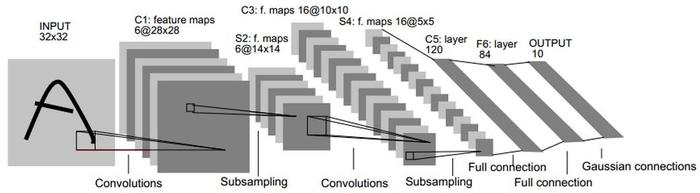
下面的代码根据 LeNET-5 模型结构在每层卷积层的卷积核数量上做了相应调整,以 MNIST 数据集为例展示了 LeNET-5Tensorflow 框架下的手写数字体识别。

模型代码 Tensorflow

1
2
3
4
5
6
7
8
9
10
11
12
13
14
15
16
17
18
19
20
21
22
23
24
25
26
27
28
29
30
31
32
33
34
35
36
37
38
39
40
41
42
43
44
45
46
47
48
49
50
51
52
53
54
55
56
57
58
59
60
61
62
63
64
65
66
67
68
69
70
71
72
73
74
75
76
77
78
79
80
81
82
83
84
85
86
87
88
89
90
91
92
93
94
95
96
97
98
99
100
101
102
103
104
105
106
107
108
109
110
111
112
113
114
115
116
117
118
119
120
121
import tensorflow as tf
from tensorflow.examples.tutorials.mnist import input_data

## 配置神经网络参数
# 输入与输出节点
INPUT_NODE = 784
OUTPUT_NODE = 10
IMAGE_SIZE = 28
NUM_CHANNELS = 1
NUM_LABELS =10
# 第一层卷积神经网络的尺寸和深度
CONV1_DEEP = 32
CONV1_SIZE = 5
# 第二层卷积神经网络的尺寸和深度
CONV2_DEEP = 64
CONV2_SIZE = 5
# 全连接层的节点个数
FC_SIZE = 1024
# 神经网络中的超参数
BATCH_SIZE = 64 # 一个训练batch中训练数据个数
LEARNING_RATE = 1e-4 # AdamOptimizer学习率
N_EPOCH = 21 # 所有训练样本训练次数

# 载入数据集
mnist = input_data.read_data_sets('MNIST_data',one_hot=True)

# 计算一共有多少个批次
n_batch = mnist.train.num_examples // BATCH_SIZE
# 定义两个placeholder
x = tf.placeholder(tf.float32, [None, INPUT_NODE]) # 28*28
y = tf.placeholder(tf.float32, [None, OUTPUT_NODE])

# 初始化权值
def weight_variable(shape):
initial = tf.truncated_normal(shape, stddev=0.1)#生成一个截断的正态分布
return tf.Variable(initial)

# 初始化偏置
def bias_variable(shape):
initial = tf.constant(0.1, shape=shape)
return tf.Variable(initial)

# 卷积层
def conv2d(x, W):
#x input tensor of shape `[batch, in_height, in_width, in_channels]`
#W filter / kernel tensor of shape [filter_height, filter_width, in_channels, out_channels]
#`strides[0] = strides[3] = 1`. strides[1]代表x方向的步长,strides[2]代表y方向的步长
#padding: A `string` from: `"SAME", "VALID"`
return tf.nn.conv2d(x, W, strides=[1,1,1,1], padding='SAME')

# 池化层
def max_pool_2x2(x):
#ksize [1,x,y,1]
return tf.nn.max_pool(x, ksize=[1,2,2,1], strides=[1,2,2,1], padding='SAME')

# 改变x的格式转为4D的格式[batch, in_height, in_width, in_channels]`
x_image = tf.reshape(x,[-1, IMAGE_SIZE, IMAGE_SIZE, NUM_CHANNELS]) # 28*28*1

# 初始化第一个卷积层的权值和偏置
W_conv1 = weight_variable([CONV1_SIZE, CONV1_SIZE, NUM_CHANNELS, CONV1_DEEP]) # 5*5的采样窗口,输入通道数是1,输出通道数是32
b_conv1 = bias_variable([CONV1_DEEP])

# 把x_image和权值向量进行卷积,再加上偏置值,然后应用于relu激活函数
h_conv1 = tf.nn.relu(conv2d(x_image, W_conv1) + b_conv1)
h_pool1 = max_pool_2x2(h_conv1) # 进行max-pooling

# 初始化第二个卷积层的权值和偏置
W_conv2 = weight_variable([CONV2_SIZE, CONV2_SIZE, CONV1_DEEP, CONV2_DEEP])#5*5的采样窗口,输入通道数是32,输出通道数是64
b_conv2 = bias_variable([CONV2_DEEP])

# 把h_pool1和权值向量进行卷积,再加上偏置值,然后应用于relu激活函数
h_conv2 = tf.nn.relu(conv2d(h_pool1, W_conv2) + b_conv2)
h_pool2 = max_pool_2x2(h_conv2) # 进行max-pooling

# 28*28的图片第一次卷积后还是28*28,第一次池化后变为14*14
# 第二次卷积后为14*14,第二次池化后变为了7*7
# 进过上面操作后得到64张7*7的平面
# (64,7,7,64)

# 获取h_pool2层的输出tensor的形状
pool_shape = h_pool2.get_shape().as_list()
NODES = pool_shape[1] * pool_shape[2] * pool_shape[3]

# 初始化第一个全连接层的权值
#上一层有7*7*64个神经元,全连接层有1024个神经元
W_fc1 = weight_variable([NODES, FC_SIZE])
b_fc1 = bias_variable([FC_SIZE])

# 把池化层2的输出扁平化为1维
h_pool2_flat = tf.reshape(h_pool2, [-1, NODES])
# 求第一个全连接层的输出
h_fc1 = tf.nn.relu(tf.matmul(h_pool2_flat, W_fc1) + b_fc1)

# keep_prob用来表示神经元的输出概率
keep_prob = tf.placeholder(tf.float32)
h_fc1_drop = tf.nn.dropout(h_fc1, keep_prob)

# 初始化第二个全连接层
W_fc2 = weight_variable([FC_SIZE, OUTPUT_NODE])
b_fc2 = bias_variable([OUTPUT_NODE])

# 计算输出
prediction = tf.nn.softmax(tf.matmul(h_fc1_drop, W_fc2) + b_fc2)
# 交叉熵代价函数
cross_entropy = tf.losses.softmax_cross_entropy(y, prediction)
# 使用AdamOptimizer进行优化
train_step = tf.train.AdamOptimizer(LEARNING_RATE).minimize(cross_entropy)
# 结果存放在一个布尔列表中
correct_prediction = tf.equal(tf.argmax(prediction,1), tf.argmax(y,1))
# 求准确率
accuracy = tf.reduce_mean(tf.cast(correct_prediction, tf.float32))

with tf.Session() as sess:
sess.run(tf.global_variables_initializer())
for epoch in range(N_EPOCH):
for batch in range(n_batch):
batch_xs,batch_ys = mnist.train.next_batch(BATCH_SIZE)
sess.run(train_step,feed_dict={x:batch_xs, y:batch_ys,keep_prob:0.7})

acc = sess.run(accuracy,feed_dict={x:mnist.test.images, y:mnist.test.labels,keep_prob:1.0})
print ("Iter " + str(epoch) + ", Testing Accuracy= " + str(acc))

AlexNet模型

简介

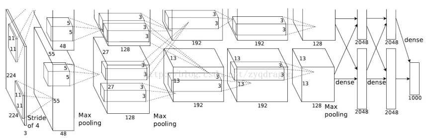
AlexNet 是2012年 ImageNet 竞赛冠军获得者 Hinton 和他的学生 Alex Krizhevsky 设计的。也是在那年之后,更多的更深的神经网路被提出,比如优秀的 VGG, GoogLeNet。

02_AlexNet

模型代码 tensorflow.contrib.slim

1
2
3
4
5
6
7
8
9
10
11
12
13
14
15
16
17
18
19
20
21
22
23
24
25
26
27
28
import tensorflow.contrib.slim as slim

def alexnet(inputs, is_training=True):
with slim.arg_scope([slim.conv2d, slim.fully_connected],
activation_fn=tf.nn.relu,
weights_initializer=tf.glorot_uniform_initializer(),
biases_initializer=tf.constant_initializer(0)):

net = slim.conv2d(inputs, 64, [11, 11], 4)
net = slim.max_pool2d(net, [3, 3])
net = slim.conv2d(net, 192, [5, 5])
net = slim.max_pool2d(net, [3, 3])
net = slim.conv2d(net, 384, [3, 3])
net = slim.conv2d(net, 256, [3, 3])
net = slim.max_pool2d(net, [3, 3])

# 数据扁平化
net = slim.flatten(net)
net = slim.fully_connected(net, 1024)
net = slim.dropout(net, is_training=is_training)

net0 = slim.fully_connected(net, num_classes, activation_fn=tf.nn.softmax)
net1 = slim.fully_connected(net, num_classes, activation_fn=tf.nn.softmax)
net2 = slim.fully_connected(net, num_classes, activation_fn=tf.nn.softmax)
net3 = slim.fully_connected(net, num_classes, activation_fn=tf.nn.softmax)

return net0,net1,net2,net3

VGG16模型

简介

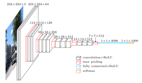
在 2014 年提出来的模型。当这个模型被提出时,由于它的简洁性和实用性,马上成为了当时最流行的卷积神经网络模型。它在图像分类和目标检测任务中都表现出非常好的结果。在 2014 年的 ILSVRC 比赛中,VGG 在 Top-5 中取得了 92.3% 的正确率。

03_VGG16

模型代码 Tensorflow

1
2
3
4
5
6
7
8
9
10
11
12
13
14
15
16
17
18
19
20
21
22
23
24
25
26
27
28
29
30
31
32
33
34
35
36
37
38
39
40
41
42
43
44
45
46
47
48
49
50
51
52
53
54
55
56
57
58
59
60
61
62
63
64
65
66
67
68
69
70
71
72
73
74
75
76
77
78
79
80
81
82
83
84
85
86
87
88
89
90
91
92
93
94
95
96
97
98
99
100
101
102
103
104
105
106
107
108
109
110
111
112
113
114
115
116
117
118
119
120
121
122
123
124
125
126
127
128
129
130
131
132
133
134
135
136
137
138
139
140
141
142
143
144
145
146
147
148
149
150
151
152
153
154
155
156
157
158
159
160
161
162
163
164
165
166
167
168
169
170
171
172
173
174
175
176
177
178
179
180
181
182
import tensorflow as tf

# 配置神经网络参数
INPUT_NODE = 150528 # 224*224*3
OUTPUT_NODE = 1000
IMAGE_SIZE = 224
NUM_CHANNELS = 3
NUM_LABELS = 1000
# 第一层卷积神经网络的尺寸和深度
CONV1_DEEP = 64
CONV1_SIZE = 3
# 第二层卷积神经网络的尺寸和深度
CONV2_DEEP = 128
CONV2_SIZE = 3
# 第三层卷积神经网络的尺寸和深度
CONV3_DEEP = 256
CONV3_SIZE = 3
# 第四层卷积神经网络的尺寸和深度
CONV4_DEEP = 512
CONV4_SIZE = 3
# 第五层卷积神经网络的尺寸和深度
CONV5_DEEP = 512
CONV5_SIZE = 3
# 全连接层的节点个数
FC_SIZE = 4096

# 计算一共有多少个批次
n_batch = mnist.train.num_examples // BATCH_SIZE
# 定义两个placeholder
x = tf.placeholder(tf.float32, [None, INPUT_NODE]) # 224*224*3
y = tf.placeholder(tf.float32, [None, OUTPUT_NODE])

# 初始化权值
def weight_variable(shape, name):
# initial = tf.truncated_normal(shape, stddev=0.1)#生成一个截断的正态分布
initial = tf.truncated_normal_initializer(stddev=0.1)
# initial = tf.contrib.layers.xavier_initializer_conv2d()
return tf.get_variable(name, shape=shape, initializer=initial)

# 初始化偏置
def bias_variable(shape, name):
# initial = tf.constant(0.1, shape=shape)
initial = tf.constant_initializer(0.1)
return tf.get_variable(name, shape=shape, initializer=initial)

# 卷积层
def conv2d(x, W):
#x input tensor of shape `[batch, in_height, in_width, in_channels]`
#W filter / kernel tensor of shape [filter_height, filter_width, in_channels, out_channels]
#`strides[0] = strides[3] = 1`. strides[1]代表x方向的步长,strides[2]代表y方向的步长
#padding: A `string` from: `"SAME", "VALID"`
return tf.nn.conv2d(x, W, strides=[1,1,1,1], padding='SAME')

# 池化层
def max_pool_2x2(x, name):
#ksize [1,x,y,1]
return tf.nn.max_pool(x, ksize=[1,2,2,1], strides=[1,2,2,1], padding='SAME', name=name)

# 改变x的格式转为4D的格式[batch, in_height, in_width, in_channels]`
x_image = tf.reshape(x,[-1, IMAGE_SIZE, IMAGE_SIZE, NUM_CHANNELS]) # 224*224*3

with tf.variable_scope('block1_conv1'):
# 初始化第一个卷积层的权值和偏置,并计算卷积结果
W_conv1 = weight_variable([CONV1_SIZE, CONV1_SIZE, NUM_CHANNELS, CONV1_DEEP], 'weights') # 3*3的采样窗口,输入通道数是3,输出通道数是64
b_conv1 = bias_variable([CONV1_DEEP], 'bias')
h_conv1 = tf.nn.relu(conv2d(x_image, W_conv1) + b_conv1)

with tf.variable_scope('block1_conv2'):
# 初始化第二个卷积层的权值和偏置,并计算卷积和池化结果
W_conv2 = weight_variable([CONV1_SIZE, CONV1_SIZE, CONV1_DEEP, CONV1_DEEP], 'weights') # 3*3采样窗口,输入通道数是64,输出通道数是64
b_conv2 = bias_variable([CONV1_DEEP], 'bias')
h_conv2 = tf.nn.relu(conv2d(h_conv1, W_conv2) + b_conv2)
h_pool1 = max_pool_2x2(h_conv2, 'pool1') # 进行max-pooling

with tf.variable_scope('block2_conv3'):
# 初始化第三个卷积层的权值和偏置,并计算卷积结果
W_conv3 = weight_variable([CONV2_SIZE, CONV2_SIZE, CONV1_DEEP, CONV2_DEEP], 'weights') # 3*3的采样窗口,输入通道数是64,输出通道数是128
b_conv3 = bias_variable([CONV2_DEEP], 'bias')
h_conv3 = tf.nn.relu(conv2d(h_pool1, W_conv3) + b_conv3)

with tf.variable_scope('block2_conv4'):
# 初始化第四个卷积层的权值和偏置,并计算卷积和池化结果
W_conv4 = weight_variable([CONV2_SIZE, CONV2_SIZE, CONV2_DEEP, CONV2_DEEP], 'weights') # 3*3采样窗口,输入通道数是128,输出通道数是128
b_conv4 = bias_variable([CONV2_DEEP], 'bias')
h_conv4 = tf.nn.relu(conv2d(h_conv3, W_conv4) + b_conv4)
h_pool2 = max_pool_2x2(h_conv4, 'pool2') # 进行max-pooling

with tf.variable_scope('block3_conv5'):
# 初始化第五个卷积层的权值和偏置,并计算卷积结果
W_conv5 = weight_variable([CONV3_SIZE, CONV3_SIZE, CONV2_DEEP, CONV3_DEEP], 'weights') # 3*3采样窗口,输入通道数是128,输出通道数是256
b_conv5 = bias_variable([CONV3_DEEP], 'bias')
h_conv5 = tf.nn.relu(conv2d(h_pool2, W_conv5) + b_conv5)

with tf.variable_scope('block3_conv6'):
# 初始化第六个卷积层的权值和偏置,并计算卷积结果
W_conv6 = weight_variable([CONV3_SIZE, CONV3_SIZE, CONV3_DEEP, CONV3_DEEP], 'weights') # 3*3采样窗口,输入通道数是256,输出通道数是256
b_conv6 = bias_variable([CONV3_DEEP], 'bias')
h_conv6 = tf.nn.relu(conv2d(h_conv5, W_conv6) + b_conv6)

with tf.variable_scope('block3_conv7'):
# 初始化第七个卷积层的权值和偏置,并计算卷积和池化结果
W_conv7 = weight_variable([CONV3_SIZE, CONV3_SIZE, CONV3_DEEP, CONV3_DEEP], 'weights') # 3*3采样窗口,输入通道数是256,输出通道数是256
b_conv7 = bias_variable([CONV3_DEEP], 'bias')
h_conv7 = tf.nn.relu(conv2d(h_conv6, W_conv7) + b_conv7)
h_pool3 = max_pool_2x2(h_conv7, 'pool3') # 进行max-pooling

with tf.variable_scope('block4_conv8'):
# 初始化第八个卷积层的权值和偏置,并计算卷积结果
W_conv8 = weight_variable([CONV4_SIZE, CONV4_SIZE, CONV3_DEEP, CONV4_DEEP], 'weights') # 3*3采样窗口,输入通道数是256,输出通道数是512
b_conv8 = bias_variable([CONV4_DEEP], 'bias')
h_conv8 = tf.nn.relu(conv2d(h_pool3, W_conv8) + b_conv8)

with tf.variable_scope('block4_conv9'):
# 初始化第九个卷积层的权值和偏置,并计算卷积结果
W_conv9 = weight_variable([CONV4_SIZE, CONV4_SIZE, CONV4_DEEP, CONV4_DEEP], 'weights') # 3*3采样窗口,输入通道数是512,输出通道数是512
b_conv9 = bias_variable([CONV4_DEEP], 'bias')
h_conv9 = tf.nn.relu(conv2d(h_conv8, W_conv9) + b_conv9)

with tf.variable_scope('block4_conv10'):
# 初始化第十个卷积层的权值和偏置,并计算卷积和池化结果
W_conv10 = weight_variable([CONV4_SIZE, CONV4_SIZE, CONV4_DEEP, CONV4_DEEP], 'weights') # 3*3采样窗口,输入通道数是512,输出通道数是512
b_conv10 = bias_variable([CONV4_DEEP], 'bias')
h_conv10 = tf.nn.relu(conv2d(h_conv9, W_conv10) + b_conv10)
h_pool4 = max_pool_2x2(h_conv10, 'pool4') # 进行max-pooling

with tf.variable_scope('block5_conv11'):
# 初始化第十一个卷积层的权值和偏置,并计算卷积结果
W_conv11 = weight_variable([CONV5_SIZE, CONV5_SIZE, CONV4_DEEP, CONV5_DEEP], 'weights') # 3*3采样窗口,输入通道数是512,输出通道数是512
b_conv11 = bias_variable([CONV5_DEEP], 'bias')
h_conv11 = tf.nn.relu(conv2d(h_pool4, W_conv11) + b_conv11)

with tf.variable_scope('block5_conv12'):
# 初始化第十二个卷积层的权值和偏置,并计算卷积结果
W_conv12 = weight_variable([CONV5_SIZE, CONV5_SIZE, CONV5_DEEP, CONV5_DEEP], 'weights') # 3*3采样窗口,输入通道数是512,输出通道数是512
b_conv12 = bias_variable([CONV5_DEEP], 'bias')
h_conv12 = tf.nn.relu(conv2d(h_conv11, W_conv12) + b_conv12)

with tf.variable_scope('block5_conv13'):
# 初始化第十三个卷积层的权值和偏置,并计算卷积和池化结果
W_conv13 = weight_variable([CONV5_SIZE, CONV5_SIZE, CONV5_DEEP, CONV5_DEEP], 'weights') # 3*3采样窗口,输入通道数是512,输出通道数是512
b_conv13 = bias_variable([CONV5_DEEP], 'bias')
h_conv13 = tf.nn.relu(conv2d(h_conv12, W_conv13) + b_conv13)
h_pool5 = max_pool_2x2(h_conv13, 'pool5') # 进行max-pooling

# 获取h_pool2层的输出tensor的形状
pool_shape = h_pool5.get_shape().as_list()
NODES = pool_shape[1] * pool_shape[2] * pool_shape[3]
keep_prob = tf.placeholder(tf.float32)

with tf.variable_scope('block6_fc1'):
# 初始化第一个全连接层的权值
W_fc1 = weight_variable([NODES, FC_SIZE], 'weights')
b_fc1 = bias_variable([FC_SIZE],'bias')
# 把池化层2的输出扁平化为1维
h_pool5_flat = tf.reshape(h_pool5, [-1, NODES])
# 求第一个全连接层的输出
h_fc1 = tf.nn.relu(tf.matmul(h_pool5_flat, W_fc1) + b_fc1)
# keep_prob用来表示神经元的输出概率
h_fc1_drop = tf.nn.dropout(h_fc1, keep_prob)

with tf.variable_scope('block6_fc2'):
# 初始化第二个全连接层
W_fc2 = weight_variable([FC_SIZE, FC_SIZE], 'weights')
b_fc2 = bias_variable([FC_SIZE], 'bias')
h_fc2 = tf.nn.relu(tf.matmul(h_fc1_drop, W_fc2) + b_fc2)
h_fc2_drop = tf.nn.dropout(h_fc2, keep_prob)

with tf.variable_scope('block6_fc3'):
W_fc3 = weight_variable([FC_SIZE, OUTPUT_NODE], 'weights')
b_fc3 = bias_variable([OUTPUT_NODE], 'bias')
h_fc3 = tf.nn.relu(tf.matmul(h_fc2_drop, W_fc3) + b_fc3)

# 计算输出
prediction = tf.nn.softmax(h_fc3)
# 交叉熵代价函数
cross_entropy = tf.losses.softmax_cross_entropy(y, prediction)
# 使用AdamOptimizer进行优化
train_step = tf.train.AdamOptimizer(LEARNING_RATE).minimize(cross_entropy)
# 结果存放在一个布尔列表中
correct_prediction = tf.equal(tf.argmax(prediction,1), tf.argmax(y,1))
# 求准确率
accuracy = tf.reduce_mean(tf.cast(correct_prediction, tf.float32))

模型代码 Keras

1
2
3
4
5
6
7
8
9
10
11
12
13
14
15
16
17
18
19
20
21
22
23
24
25
26
27
28
29
30
31
32
33
34
35
36
37
38
39
40
41
42
43
from keras import Sequential
from keras.layers import Dense, Activation, Conv2D, MaxPooling2D, Flatten, Dropout
from keras.layers import Input
from keras.optimizers import SGD

model = Sequential()

# BLOCK 1
model.add(Conv2D(filters = 64, kernel_size = (3, 3), activation = 'relu', padding = 'same', name = 'block1_conv1', input_shape = (224, 224, 3)))
model.add(Conv2D(filters = 64, kernel_size = (3, 3), activation = 'relu', padding = 'same', name = 'block1_conv2'))
model.add(MaxPooling2D(pool_size = (2, 2), strides = (2, 2), name = 'block1_pool'))

# BLOCK2
model.add(Conv2D(filters = 128, kernel_size = (3, 3), activation = 'relu', padding = 'same', name = 'block2_conv1'))
model.add(Conv2D(filters = 128, kernel_size = (3, 3), activation = 'relu', padding = 'same', name = 'block2_conv2'))
model.add(MaxPooling2D(pool_size = (2, 2), strides = (2, 2), name = 'block2_pool'))

# BLOCK3
model.add(Conv2D(filters = 256, kernel_size = (3, 3), activation = 'relu', padding = 'same', name = 'block3_conv1'))
model.add(Conv2D(filters = 256, kernel_size = (3, 3), activation = 'relu', padding = 'same', name = 'block3_conv2'))
model.add(Conv2D(filters = 256, kernel_size = (3, 3), activation = 'relu', padding = 'same', name = 'block3_conv3'))
model.add(MaxPooling2D(pool_size = (2, 2), strides = (2, 2), name = 'block3_pool'))

# BLOCK4
model.add(Conv2D(filters = 512, kernel_size = (3, 3), activation = 'relu', padding = 'same', name = 'block4_conv1'))
model.add(Conv2D(filters = 512, kernel_size = (3, 3), activation = 'relu', padding = 'same', name = 'block4_conv2'))
model.add(Conv2D(filters = 512, kernel_size = (3, 3), activation = 'relu', padding = 'same', name = 'block4_conv3'))
model.add(MaxPooling2D(pool_size = (2, 2), strides = (2, 2), name = 'block4_pool'))

# BLOCK5
model.add(Conv2D(filters = 512, kernel_size = (3, 3), activation = 'relu', padding = 'same', name = 'block5_conv1'))
model.add(Conv2D(filters = 512, kernel_size = (3, 3), activation = 'relu', padding = 'same', name = 'block5_conv2'))
model.add(Conv2D(filters = 512, kernel_size = (3, 3), activation = 'relu', padding = 'same', name = 'block5_conv3'))
model.add(MaxPooling2D(pool_size = (2, 2), strides = (2, 2), name = 'block5_pool'))

model.add(Flatten())
model.add(Dense(4096, activation = 'relu', name = 'fc1'))
model.add(Dropout(0.5))
model.add(Dense(4096, activation = 'relu', name = 'fc2'))
model.add(Dropout(0.5))
model.add(Dense(1000, activation = 'softmax', name = 'prediction'))

model.summary()

Keras.application中的VGG16模型

VGG16模型的权重由ImageNet训练而来。该模型在Theano和TensorFlow后端均可使用,并接受channels_first和channels_last两种输入维度顺序,模型的默认输入尺寸是224x224。

1
2
3
import keras

model = keras.applications.vgg16.VGG16(include_top=True, weights='imagenet', input_tensor=None, input_shape=None, pooling=None, classes=1000)

参数说明

  • include_top:是否保留顶层的3个全连接网络
  • weights:None代表随机初始化,即不加载预训练权重。’imagenet’代表加载预训练权重
  • input_tensor:可填入Keras tensor作为模型的图像输出tensor
  • input_shape:可选,仅当include_top=False有效,应为长为3的tuple,指明输入图片的shape,图片的宽高必须大于48,如(200,200,3)

返回值

  • pooling:当include_top=False时,该参数指定了池化方式。None代表不池化,最后一个卷积层的输出为4D张量。‘avg’代表全局平均池化,‘max’代表全局最大值池化。
  • classes:可选,图片分类的类别数,仅当include_top=True并且不加载预训练权重时可用。
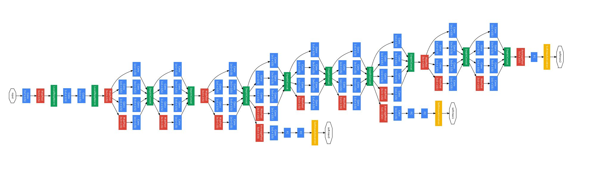
GoogleNet/Inception

04_GoogleNet

ResNet

DenseNet

坚持原创技术分享,您的支持将鼓励我继续创作!